Simulated Broker

The SimBroker implements the Broker interface just like any other implementation. You use the SimBroker class (short for Simulated Broker) both for the back testing and forward testing stages.

See also the four stages for more background about the different stages when developing trading strategies.

SimBroker can simulate a wide range of brokers and exchanges. Besides several configuration parameters that are available, the behavior can be further extended by providing custom models for trading, fee and account modelling.

Usage

The instantiation of a SimBroker is surprisingly simple if the default settings suit your needs:

val broker = SimBroker()

This is also the configuration you get when you create an instance of Roboquant and don’t specify a broker at all.

However, you can overwrite many of the default values. Common use cases are:

you don’t trade in USD but in some other currency
you want to simulate a MarginAccount and not the default CashAccount
you want to apply custom fees and pricing logic

So a more custom-configured version of the SimBroker can be instantiated using:

val broker = SimBroker(
    initialDeposit = Wallet(10_000.EUR), // how much to initially deposit into the account
    baseCurrency = Currency.EUR, // currency to use for reporting
    feeModel = PercentageFeeModel(), // model to use to calculate fees, commissions, etc
    accountModel = MarginAccount(), // type of account to model, like a Cash or Margin account
    pricingEngine = SpreadPricingEngine() // engine to use to calculate the final price of a trade
)

If you are trading specific markets, like FOREX, you most likely want to use customize the configuration. The default values, like those selected for spreads, might not be representative for those types of liquid markets.

The initial deposit is the cash that is deposited at the opening of an account. Any time the SimBroker is reset, the account will be reset to this initial deposit. Typically, the initial deposit is denoted in a single currency, like a $50,000.00 USD account. But this is not a hard requirement and with SimBroker you can use a multi-currency initial deposit if you prefer. However, there is always only one baseCurrency.

Order Execution

When an order is placed at the SimBroker, the following rules apply:

Create-orders only get executed if there is a known price for the underlying asset. Till an event occurs that has that price action available, the order will remain in its INITIAL state and will not be executed.
Modify-orders will always get executed, even if there is no known price for the asset.
Any TIF (Time In Force) enforcement of order execution will only start after an order has been accepted. So an order in INITIAL state will not expire, and time-based TIF will only start counting after it has been accepted.
Modify-orders will always be processed BEFORE create-orders. So if you send a CancelOrder and MarketOrder for the same asset, the CancelOrder is guaranteed to be processed first in the SimBroker.
Create- and modify-orders will be processed based on a FIFO (first-in-first-out) basis, so older orders are processed first.
Once an order is closed, it cannot be opened again.
When an order is placed at time t, the order-execution will start at time t+1. This avoids looking-ahead bias.

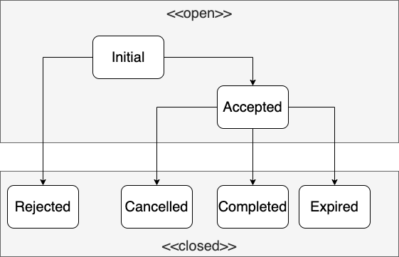
The following diagram shows the possible OrderStatus transitions:

Customize SimBroker

Custom models are a way to further customize the SimBroker and ensure it closely mimics the behavior of your real broker.

If you don’t take any type of trading cost into account, your profitable strategy in back-test might turn out not to be that profitable in live trading. When in doubt, better to be on the safe side and configure the cost to be slightly higher than expected.

The following three types of models can be implemented if the default ones that come with roboquant are not sufficient:

PricingEngine — Calculate the price to use for a trade. It can be used to simulate the following type of trading cost:
- Spread (difference between the buy- and sell-price)
- Slippage (large orders will require multiple trades against different prices)
FeeModel — Model the transaction-related fees and commissions. Trading cost to take into consideration:
1. Broker commission fees
2. Borrowing cost when shorting
3. Storage & custodial fees
4. Exchange fees and/or rebates
AccountModel — Calculate the available buying-power based on margins, open orders, cash and open positions.

Before implementing your own model, it is advisable to check if the default-included models with their configuration options aren’t sufficient. Below the available models with some examples of their configuration parameters:

// Account Models
val accountModel1 = CashAccount(minimum = 1_000.0)
val accountModel2 = MarginAccount(
    initialMargin = 0.5,
    maintenanceMarginLong = 0.3,
    maintenanceMarginShort = 0.2,
    minimumEquity = 10_000.0
)

// Fee models
val feeModel1 = PercentageFeeModel(0.01) // 1% fee
val feeModel2 = NoFeeModel() // no additional fees apply

// Pricing engines
val pricingEngine1 = SpreadPricingEngine(spread = 5.bips, priceType = "OPEN")
val pricingEngine2 = NoCostPricingEngine(priceType = "CLOSE")

Limitations

Like any simulation, SimBroker also has limitations compared to live trading. It is important to realize this and take appropriate measures when possible:

The default cost calculations become less realistic if you trade large sizes compared to overall daily volume. As a rule of thumb: don’t underestimate the additional costs like spread, slippage and commissions and better be on the safe side.
Order types might behave slightly different between SimBroker and different real brokers. If possible, perform extensive paper trading testing to see if your solution still performs as expected.
The buying power and margin calculations might differ. Again, be on the safe side and use higher margin requirements in the SimBroker than required by your actual broker.

PricingEngine

The PricingEngine determines the price that is used for a trade execution. There are default ones included, but you can also easily implement your own:

class MyPricingEngine : PricingEngine {

    inner class MyPricing(val action: PriceAction) : Pricing {

        override fun marketPrice(size: Size): Double {
            return when (action) {
                is PriceQuote -> if (size.isPositive) action.askPrice else action.bidPrice
                is OrderBook -> if (size.isPositive) action.bestOffer else action.bestBid
                else -> action.getPrice()
            }
        }

    }

    override fun getPricing(action: PriceAction, time: Instant): Pricing {
        return MyPricing(action)
    }

}

Account Models

Account models allow you to model the amount of buying-power for different types of accounts, like a Cash Account or Margin Account when using the SimBroker. Buying-power represents the amount of money available for trading.

Out of the box roboquant comes with two account models that cater for the most common account types:

CashAccount; account that doesn’t have any leverage or margin available.
MarginAccount; account that has (configurable) initial and maintenance margin requirements.

Cash Accounts

Cash accounts can be modelled using the CashAccount. This model is also the default if you don’t provide a BuyingPowerModel when instantiating a SimBroker.

CashAccount bases the buying power only on the available cash, and no margin is calculated and no leverage is used. So cash and buying power are equal, however cash can contain multiple currencies while the buying power is always converted to the base currency of the account.

Although roboquant doesn’t stop you from using this model even when shorting assets, it is not advised to do so.

The below table shows an example using the default CashAccount when trading in different currencies, EUR and USD in this case.

Time	Action	Cash	Positions	Equity	Buying Power	Unrealized PnL	Realized PnL
1	open account with €10,000	€10,000	0	€10,000	€10,000	0	0
2	buy ABC 40 @ €100	€6,000	€4,000	€10,000	€6,000	0	0
3	price ABC drops to €75	€6,000	€3,000	€9,000	€6,000	-€1,000	0
4	sell ABC -40 @ €75	€ 9,000	0	€ 9,000	€9,000	0	-€1,000
5	buy XYZ 25 @ $200	€9,000 -$5,000	$5,000	€9,000	€4,500	0	-€1,000
6	price XYZ raises to $240	€9,000 -$5,000	$6,000	€9,000 $1,000	€4,500	$1,000	-€1,000
7	sell XYZ -25 @ $240	€9,000 $1,000	0	€9,000 $1,000	€9,900	0	-€1,000 $1,000

Margin Accounts

Margin accounts can be modelled using the MarginAccount. This model supports:

Initial margin (aka leverage)
Maintenance margin, with support for different maintenance percentages for long and short positions
Minimum amount of equity that cannot be used as margin (to stay away from margin calls)

All margin calculations are based on the equity of the account, and not just the cash. And although in the below tables the (maintenance) margin is shown, it is actually not exposed. Only the buying-power value is available through the account object.

The calculations for the buying-power look roughly like this in pseudocode:

long_margin = long_positions * maintenance_margin_long
short_margin = short_positions * maintenance_margin_short
excess_margin = equity - long_margin - short_margin - minimum_equity
buying_power = excess_margin * ( 1 / initial_margin)

The following table shows an example for long trading with a margin account in the Japanese Yen, using the following (default) values:

initial margin: 50%
maintenance margin: 30% (both for long and short positions)
no minimum equity is required

Also, there are no commissions or other costs associated with the transactions. This is not a recommended approach, but just used here to make it a bit simpler to comprehend.

Time	Action	Cash	Portfolio	Margin	Equity	Buying Power	Unrealized PnL	Realized PnL
1	open account with ¥1,000,000	¥1,000,000	0	0	¥1,000,000	¥2,000,000	0	0
2	buy ABC 500 @ ¥1,000	¥500,000	¥500,000	¥150,000	¥1,000,000	¥1,700,000	0	0
3	ABC drops to ¥500	¥500,000	¥250,000	¥75,000	¥750,000	¥1,350,000	-¥250,000	0
4	buy ABC 2000 @ ¥500	-¥500,000	¥1,250,000	¥375,000	¥750,000	¥750,000	-¥250,000	0
5	ABC drops to ¥400	-¥500,000	¥1,000,000	¥300,000	¥500,000	¥400,000	-¥500,000	0
6	sell ABC -2500 @ ¥400	¥500,000	0	0	¥500,000	¥1,000,000	0	-¥500,000

The following table shows another example, but this time shorting on a USD margin account. It uses the same default values for the margin calculations as the above table.

Time	Action	Cash	Positions	Margin	Equity	Buying Power	Unrealized PnL	Realized PnL
1	open account with $20,000	$20,000	0	0	$20,000	$40,000	0	0
2	sell XYZ -50 @ $200	$30,000	-$10,000	$3,000	$20,000	$34,000	0	0
3	price XYZ raises to $300	$30,000	-$15,000	$4,500	$15,000	$21,000	-$5,000	0
5	sell XYZ -50 @ $300	$45,000	-$30,000	$9,000	$15,000	$12,000	-$5,000	0
6	buy XYZ 100 @ $300	$15,000	0	0	$15,000	$30,000	0	-$5,000

Order impact on Buying Power

The following order-rules apply when calculating the buying power:

Until an order is accepted (so in INITIAL state), it doesn’t impact margin or buying power.
Open orders that reduce a position size do not require buying power. So you can always close a position, both short and long positions.
Once an order has been accepted, it will not be cancelled due to lack of buying power.
An order in a closed state doesn’t impact margin or buying power (so similar to the INITIAL state)

Not all rules are currently implemented yet.

Margin Calls

A negative value for BuyingPower indicates a possible margin call situation. However, roboquant doesn’t interrupt the back-test if that condition happens. However, if the DefaultPolicy is used, it will guarantee that no new positions will be opened. Only the decrease of positions is allowed if there is insufficient buying-power available.

If you are interested in detecting these conditions, best to configure a metric that logs the BuyingPower at each step and evaluate that metric after the run.

Always be very conservative about the amount of margin being available. Stay as far away from margin calls as possible, since these are typically manual broker processes that cannot be automated in an algo-trading strategy.

Realized profit

Open positions hold unrealized profit. As soon as a trade happens, some of this unrealized profit can become realized profit.

The following table shows the logic that is applied for long positions:

Position before	Trade	Position after	Realized PnL	Remark
0	10 @ $104.0	10 @ $104.0	$0.0	Open position
10 @ $100.0	-10 @ 104.0	0	$40.0	Close position
10 @ $100.0	10 @ 104.0	20 @ $102.0	$0.0	Increase position
10 @ $100.0	-20 @ 104.0	-10 @ $104.0	$40.0	Reverse position

Position before

Trade

Position after

Realized PnL

Remark

10 @ $104.0

$0.0

Open position

10 @ $100.0

-10 @ 104.0

$40.0

Close position

10 @ $100.0

10 @ 104.0

20 @ $102.0

$0.0

Increase position

10 @ $100.0

-20 @ 104.0

-10 @ $104.0

$40.0

Reverse position

The same logic applies to short positions:

Position before	Trade	Position after	Realized PnL	Remark
0	-10 @ $104.0	-10 @ $104.0	$0.0	Open position
-10 @ $100.0	10 @ 104.0	0	-$40.0	Close position
-10 @ $100.0	-10 @ 104.0	-20 @ $102.0	$0.0	Increase position
-10 @ $100.0	20 @ 104.0	10 @ $104.0	-$40.0	Reverse position

Position before

Trade

Position after

Realized PnL

Remark

-10 @ $104.0

$0.0

Open position

-10 @ $100.0

10 @ 104.0

-$40.0

Close position

-10 @ $100.0

-10 @ 104.0

-20 @ $102.0

$0.0

Increase position

-10 @ $100.0

20 @ 104.0

10 @ $104.0

-$40.0

Reverse position